Analyze results of the repair

After selecting a particular protein from the queue (or the database of repaired nontrivial proteins) users can view all information about it in the Results pages, which can be divided into following categories:

  1. Job status
  2. General information about modelling process and results (templates used, final model scores, rebuilt protein visualization):
    1. Summary
    2. Templates
    3. Downloads list, with both gzipped models, and modelling alignments
    4. Job log
  3. Information about modelling process and results in the case of entangled structures


  1. Job status
    • Basic information about the job – shown in Fig. 1; contains project name, PDB ID (for structures from the PDB database), the unique job id and current status (part of the information can be displayed as soon as the models are created, before the entanglement checking).
    • Fig. 1 Basic information about the job: project name, PDB ID (for structures from the PDB database), the unique job id and current status.

    • There are three possible status icons:
      1. Finished
        indicates that the job finished without any problems - neither during modelling, nor with the entanglement check.

      2. Modelled
        indicates that the modelling part of the job finished without any problems - entanglement check is in progress.

      3. Running
        the job is being processed, with no obstacles so far. If modelling is still ongoing, the Results page contains only the Job log. After the modelling is done, and entanglement profiles are being calculated, basic information about the models is available (all the panels described in General information section).

      4. Error
        job could not finish due to some error. Job log indicates at which stage of the workflow the job has crashed.

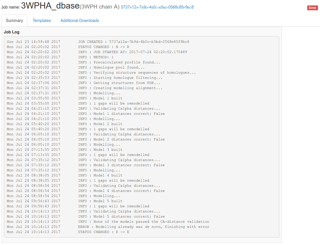
        Fig. 2 Example of failure: Job log of modelling gone wrong.

        If the modelling has been completed (e.g. only the entanglement detection failed) all the information calculated prior to the failure is available (all the panels described in General information section).

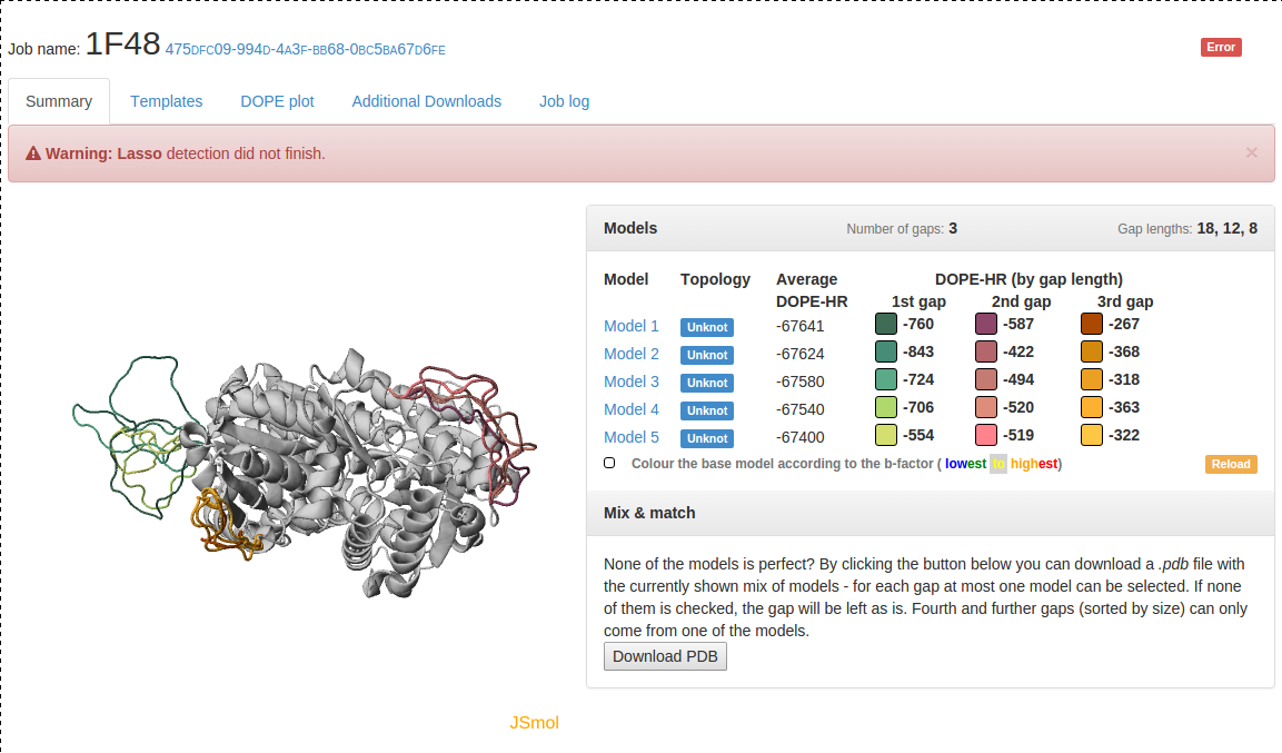
        Fig. 3 Example of failure: Modelling went without a hitch, but some problems were encountered during entanglement calculation.


  2. General information about modelling process and results
    • Summary – this screen is shown focused on elements common to all structures in Fig. 4 below; it contains:

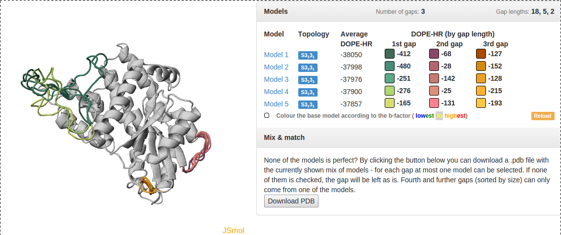
      Fig. 4 An example of data presentation for a knotted protein with PDB ID 1ual repaired using GapRepairer. Applet in top left: graphical representation of protein in JSmol. Top right: DOPE-HR scores for each model/gap combination and control panel for applet. Bottom right: Download button for a structure created from multiple models.

      • list of all the models sorted by ascending average DOPE-HR (top right). For each model DOPE for up to three gaps is shown separately, with colored squares allowing to hide and show a given gap. The fourth and further gaps are clustered for each model, and can only be displayed for one model at a time. This panel containes also a Reload button (to return the display to the starting appearance) and a button to colour the base structure according to the b-factor (if specified in the PDB file). Each model name links to the .pdb file containing its structure.
      • The JSmol applet presenting the graphic representation of the uploaded structure and up to 5 models with the reconstructed gaps (top left). Different colours correspond to those used in model panel on the right - that is indicate to which model does this particular reconstruction belong to.
      • Fig. 5 An example of structure visualization for a knotted protein with PDB ID 4mcb repaired using GapRepairer. Left: Electron density map (σ=1, 1.5Å around the structure) overlay. Right: Difference electron density map (σ=3, 3Å around the structure) overlay.

      • Where available, the electron density maps (2mFo-DFc and mFo-DFc, both in two versions) or density maps for Cryo-EM structures (based on EMBL-EBI EDS server) are displayed on the visualization of modelled structures. Note that, if the target structure provided by the user contains crystallograpic cell and space group definitions, this data is available in the final model files.
      • Mix & match panel, where for a protein with multiple gaps you can download a structure with gaps filled by parts from different models (right). The structure downloaded will be the currently displayed one - that is any gaps that have no model displayed will remain empty. When more than one model is selected for a given gap only the highest scoring one (based on average DOPE-HR) will be used - i.e. when both Model 2 and Model 4 are selected, the gap will be filled based on Model 2.

    • Fig. 6 Templates panel: statistics pertaining to each selected template and pairwise alignment to the target. Amino acids in the alignment coloured according to the scheme used in I-Tasser. Modelled gaps indicated by a gray highlight, with three largest gaps underlined additionally in red.

    • Templates – this screen contains information about the homologues chosen for the modelling (as shown in the Fig. 11 below):
      • each template described using its PDB ID; selected protein chain; topology; statistics based on the pairwise sequence alignment to the target: sequence identity, gap coverage, sequence identity in gaps; RMSD between superposed structures; and aforementioned pairwise alignment in a scrollable window with gaps marked by a grey highlight and three largest additionally underlined in red (all shown in Fig. 3 above).
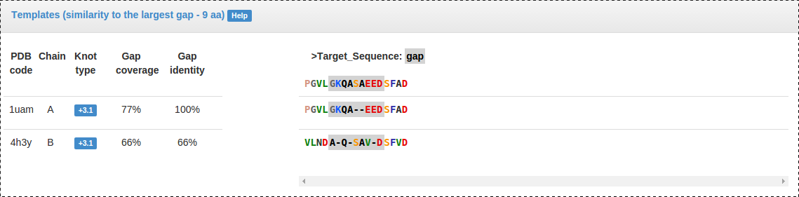
      • Fig. 7 Gap panel: present for each gap being repaired, specifies gap coverage and identity for each template, and the multiple sequence alignment used for homologous modelling.

      • Similarity between the target and selected templates within each gap. Sequences are presented as a multiple sequence alignment used by MODELLER, and statistics are calculated based on this alignment ( Fig. 7 above).
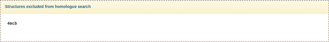
      • Fig. 8 Excluded structures: panel which lists proteins excluded by the user - not necessairly proteins which would be used if not for this exclusion. Syntax mirrors the one used in the input field - if chain was specified it is added for a given PDB ID after the colon.

      • List of proteins/chains excluded from template search (Fig. 8 above) where such were specified (option available under the Advanced options tab in the Repair form).

    • Additional downloads – provides links to the alignment used by MODELLER and a .tar.gz archive containing all the models (Fig. 9).
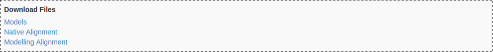
    • Fig. 9 Download tab: links to model files and alignment used for modelling.
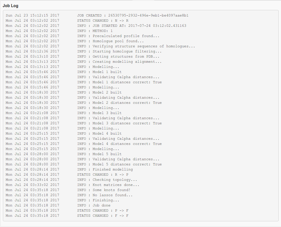

    • Job log – lists all steps of the process with timestamps, and additional parameters specified by the user (Fig. 10).
    • Fig. 10 Job log.

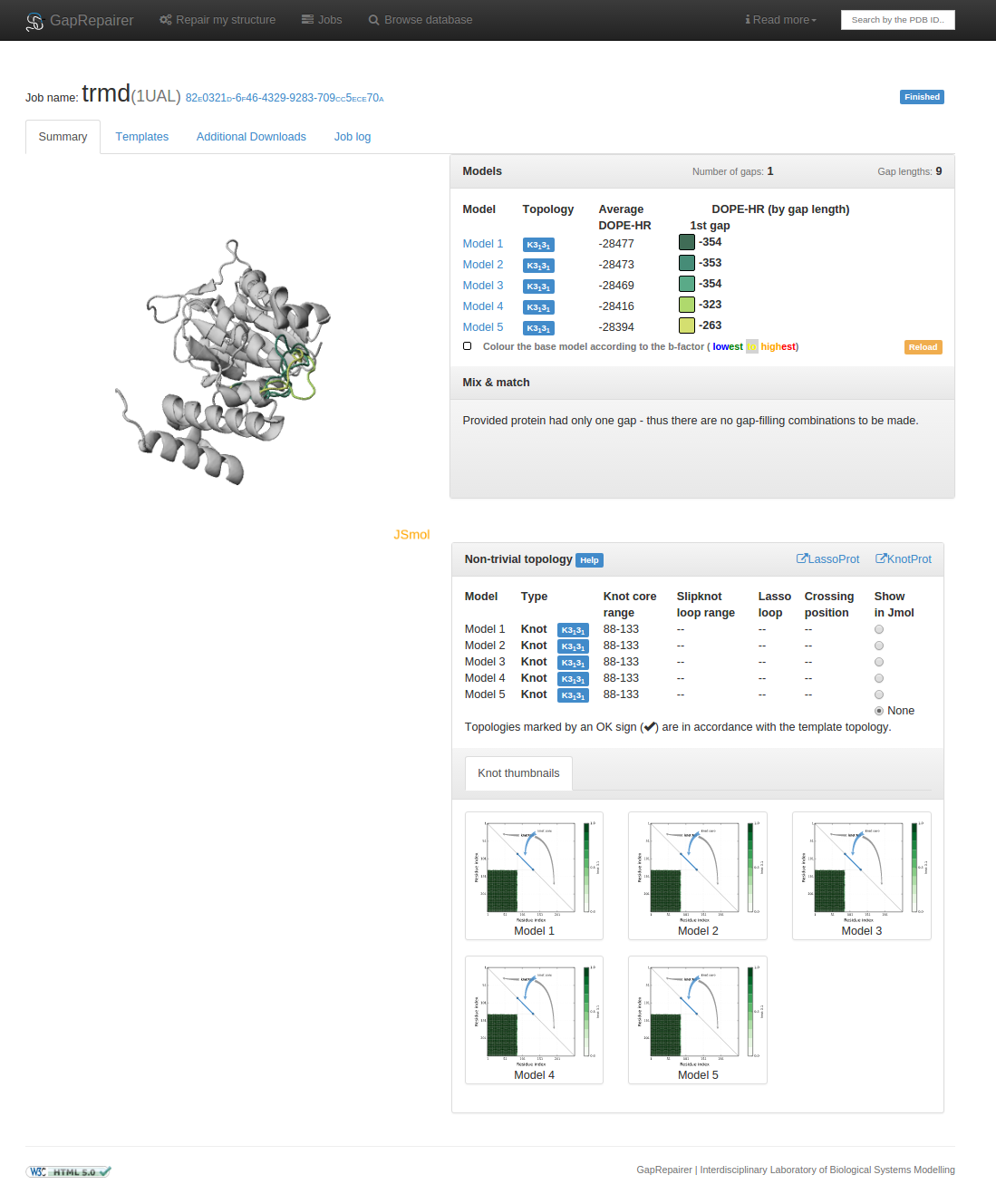
    Fig. 11 An example of data presentation for a knotted protein with PDB ID 1ual repaired using GapRepairer. Applet in top left: graphical representation of protein in JSmol. Top right: DOPE-HR scores for each model/gap combination and control panel for applet. Middle right: detailed data about knots/slipknots and lassos formed by backbone subchains. Bottom right: diagram presenting a topology matrix for the models.

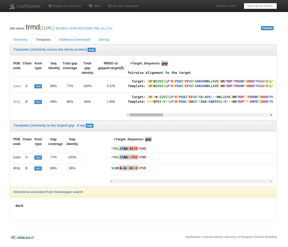
    Fig. 12 An example of selected homologues presentation for a knotted protein with PDB ID 1ual repaired using GapRepairer. First panel shows averaged statistics for each template based on a pairwise sequence alignment with target. Middle panel presents multiple sequence alignment used for modelling missing residues. Last panel lists structures excluded from the homologue search (in this case: all chains form the protein with PDB ID 4mcb).


  3. Entangled proteins
  4. For protein chains with any kind of entanglement additional panel is available on the summary page:

    • Entanglement table (Fig. 13), which lists all models with their type (Knot/Slipknot/Lasso); fingerprint; and position. Radio button on the right hand side displays knot/lasso details on the applet in the top left of the page (Fig. 14) and both marks by a blue highlight and opens in a larger panel respective thumbnail (Fig. 15). For models with both knot and lasso, they are listed in consecutive lines.

    • Knot thumbnails (where applicable - full Summary page for a knotted protein shown in Fig. 16 below), tiles containing topology matrix for each nontrivially folded model (images enlarge on the left side of the screen after clicking them - Fig. 17).
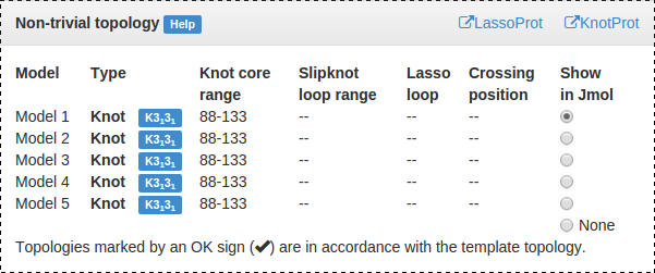
    • Fig. 13 Table detailing location of the outmost knot/slipknot for each model. Radio button in the last column displays this entanglement in the JSmol applet, and enlarges and highlights the corresponding matrix.

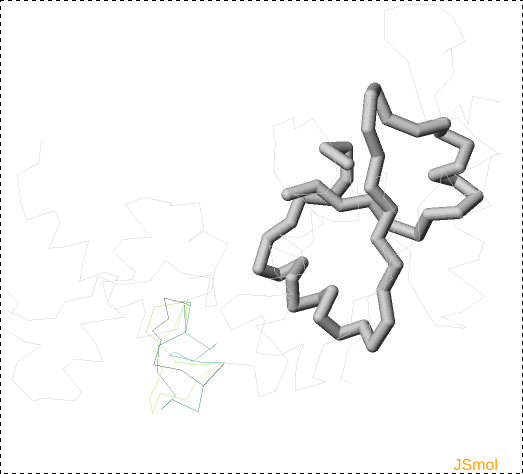
      Fig. 14 Knot location visualized in the JSmol applet: knot core (chain segment that elongated by one aminoacid would already form the knot) is show as the thickest line coloured blue, slipknot loop (not present in this picture) has medium thickness and yellow colour, and rest of the protein is a thin grey line.

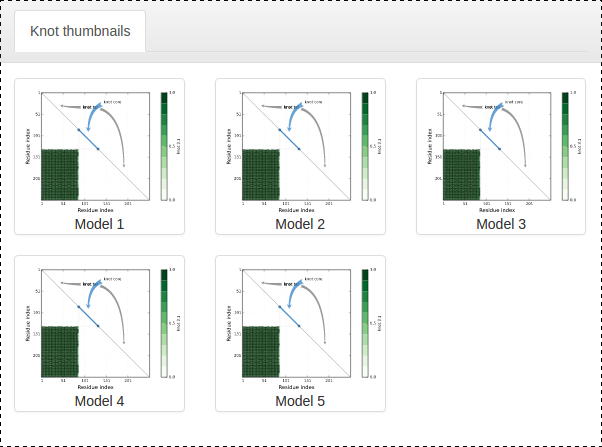
      Fig. 15 Topology matrices which indicate presence (or absence) of a particular entanglement, were the chain cut only to the segment between given position (eg. if position (35,160) is coloured green chain contains a 31 knot somewhere between 35th and 160th amino acid).


    • Lasso thumbnails (where applicable - full Summary page for a lasso protein shown in Fig. 19 below), tiles containing spherically presented lasso from each model containing one, with the crossing position colored in (images enlarge on the left side of the screen after clicking them).
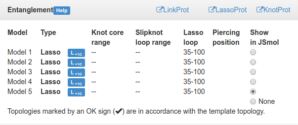
    • Fig. 16 Table detailing location of the outmost knot/slipknot for each model. Radio button in the last column displays this structure in the JSmol applet, and enlarges and highlights the corresponding matrix.

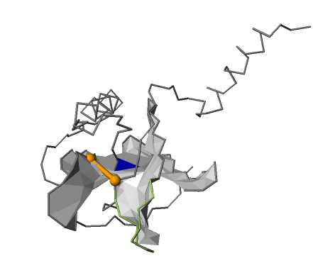
      Fig. 17 Lasso location visualized in the JSmol applet. Cystein bridge that closes the lasso loop is imagined in yellow, surface of the loop is formed by gray triangles with the crossing coloured blue.

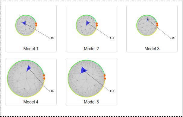
      Fig. 18 Outmost lasso loop of a model visualized as a circle, with the crossings marked in blue and annotated by the number in the protein chain of the amino acid closest to the crossing on the threaded fragment.

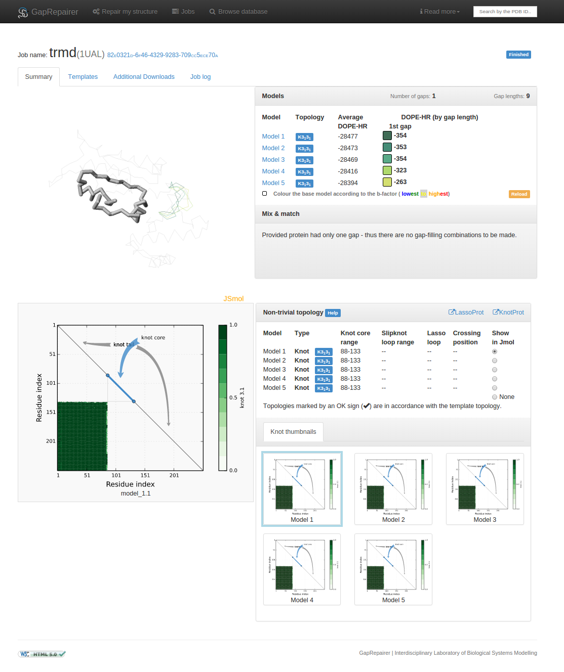
    Fig. 19 An example of data presentation for a knotted protein with PDB ID 1ual repaired using GapRepairer.

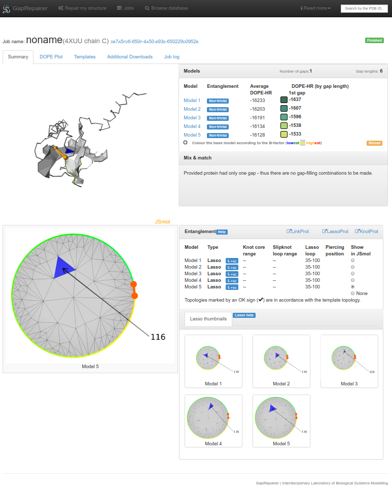
    Fig. 20 An example of data presentation for a protein with PDB ID 4xuu (chain C), which contains a lasso, repaired using GapRepairer.


GapRepairer | Interdisciplinary Laboratory of Biological Systems Modelling